
Dealing with complex Excel databases or other advanced tasks may require using certain advanced features like TEXTAFTER, an essential tool for advanced Excel users. It helps extract data to the right of a particular character or word. You can use TEXTAFTER to return any text that occurs after giving a substring or delimiter. Also, the same feature, TEXTAFTER, can return texts after several recurrences of some delimiters.
How do you use the HEREAFTER feature or TEXTAFTER in Excel? This article will show you how to do it so you can get back to work fast.
Use TEXTAFTER in Excel
Excel’s TEXTAFTER feature will save you a lot of stress by helping you return characters occurring after a specified string, and you will need it if you need to find characters lying within a string.
First, below is the syntax format you need for executing the TEXTAFTER feature:
=TEXTAFTER(text,delimiter,[instance_num], [match_mode], [match_end], [if_not_found])The syntax above has two required arguments which are text and delimiter.
The ‘text’ argument represents the text or the cell name containing the text you need to find in the database, while the ‘delimiter’ represents the last character just before the point you want to search.
Other arguments in the syntax are secondary, but they will help you find texts. However, you can still ignore them, but you should understand what they represent too.
- Instance_num represents the delimiter after which you want to extract. The value is n=1, by default. However, a negative instance number means the system will search from the end.
- Match_mode is a determiner that checks if the search is case-sensitive. It can only take two values which are 0 and 1. 0 means the search is case-sensitive, and 1 means it is not. This argument is set to 0 by default. The system will assume your search is case-sensitive unless it is 1.
- Match_end takes the end of the text as a delimiter. It can also take only two values, 0 and 1, like match_mode. 0 is the default value, and it will not treat the end of the text as a delimiter, while 1 does otherwise.
- If_not_found is the value you want the search to display if it does not find a match. You can enter anything in this field, but the system will return #N/A by default if you did not set it up.
Important Note: The TEXTAFTER feature is not available on all Excel versions. It is only available on Office 365. If your version does not have this feature, you can check out an online Excel version here.
Example 1: Illustration with the Required Arguments Only
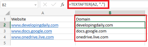
This example above used the two required arguments - text and delimiter. The text is the cell reference A2, and the delimiter is the full stop. Note that there is a comma sign after each argument in the formula. The delimiter is also within quotation marks.
The formula =TEXTAFTER(A2, “.”) implies that I want to search for all the texts after the first full-stop sign in Cell A2, A3, and A4, as seen in the image.
Here, I didn’t use the optional arguments, so the system used the defaults values for each as follows:
- Instance_num is 1, by default, meaning the search will return all the texts after the first full-stop sign.
- Match_mode is 0, meaning it is case-sensitive.
- Match_end is 0 and will not take the end of the text as a delimiter.
Example 2: Illustration with Instance_num
Adding an instance number to the illustration in example 1 will change the result. For instance, if I use an instance number of 2, the worksheet will return the text after the second appearance of the delimiter. It will show the text after the second full stop, as seen below.

Also, changing the instance number to -1 will make the system search from the right and return the text after the first delimiter from the right side.

In the same way, if the instance number is -3, the formula will start counting from the right because of the minus sign and return the texts after the third delimiter. Remember, the delimiter in this illustration is the full-stop sign.
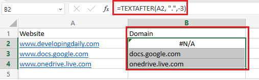
As you can see, cell B2 returned with #N/A since A2 does not have up to three full-stop signs.
Example 3: Illustration with Instance_not, found
The TEXTAFTER formula is =TEXTAFTER(text,delimiter,[instance_num], [match_mode], [match_end], [if_not_found])
You can state an if_not_found condition while skipping other optional arguments, and in this illustration, it will assign default values to match_mode and math_end.
To do this, I will add commas in their place, and the system will set both arguments to their default values.
- =TEXTAFTER(text,delimiter,[instance_num],, [match_end], [if_not_found]) will skip match_mode.
- =TEXTAFTER(text,delimiter,[instance_num], [match_mode],, [if_not_found]) will skip match_end.
- =TEXTAFTER(text,delimiter,[instance_num],,, [if_not_found]) will skip both arguments. Note that the number of commas will increase depending on the number of optional arguments you want to skip.
To use if_not_found argument in this illustration while skipping match_mode and match-end, we will use the formula:
=TEXTAFTER(A2,.,“-3”,,,“No Value”)

The formula above will search the right and returns the text after the third appearance of the delimiter. Since A2 does not have up to three full stop signs, it returned with the if_not_found command input.
Conclusion
The TEXTAFTER command saves time, but you may return error reports if you do not input the formula appropriately. Ensure you used quotations where necessary and that your office version is 365.
You may also like to read:
How To Rename a Table In Excel
Best Automation Software Tools
How To Create Dependent Drop-down List in Excel
How to Switch First and Last Names in Excel with Comma
How to Insert a Signature in Excel
How To Remove Empty Cells In Excel
How To Change Date Format In Excel To dd/mm/yyyy